

post we will provide solution to the below listed questions:
1.How to Use INDEX+MATCH With Multiple Criteria.
2.How to Lookup a value With Multiple Criteria.
3.How to find the row number in excel with multiple match Criteria.
| Lookup Table | |||
|---|---|---|---|
| Company Id | Location | Turnover | Rating |
| 100 | India | 1 | AA |
| 101 | US | 3 | BB |
| 102 | UK | 1 | AA |
| 103 | India | 2 | A+ |
| 104 | Japan | 1 | AAA |
| 105 | India | 2 | BBB |
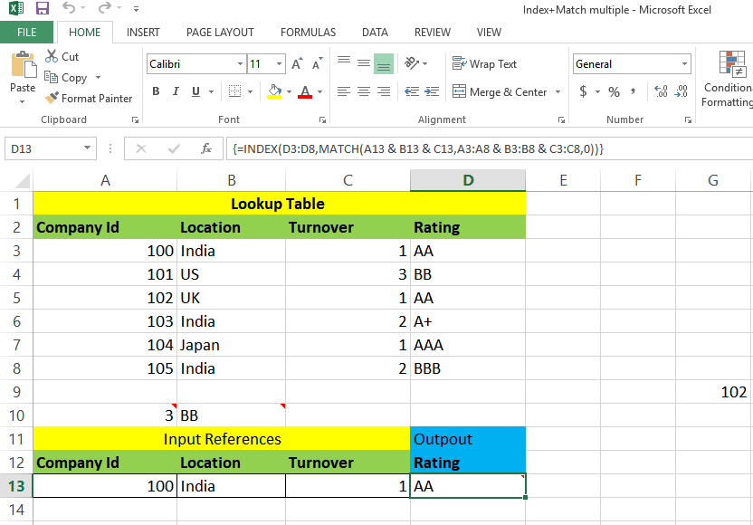
Problem Statement: Lookup the value of rating from Lookup table where
1.Company Id=100
2.Location= India
3.Turnover=1
Solution: You can download example sheet for details.

Final Function will be {=INDEX(D3:D8,MATCH(E13 & F13 & G13,A3:A8 & B3:B8 & C3:C8,0))} and it will return AA
Let us see it in details:
This is very common requirement when you are working on data analysis or you are creating some automated script or if you are trying create some dashboard for financial calculations.
Before Reading this article, I am assuming visitors are aware of INDEX, MATCH and VLOOKUP.
I will use INDEX and MATCH combination to solve our problem. Let us discuss briefly these function before we use it:
INDEX function’s syntax- INDEX(array, row_num, [column_num])
If both row_num and column_num parameters are used, the INDEX function returns the value in the cell at the intersection of the specified row and column.
Example:
| Lookup Table | |||
|---|---|---|---|
| Company Id | Location | Turnover | Rating |
| 100 | India | 1 | AA |
| 101 | US | 3 | BB |
| 102 | UK | 1 | AA |
| 103 | India | 2 | A+ |
| 104 | Japan | 1 | AAA |
| 105 | India | 2 | BBB |
INDEX(A3:C8,3,1) will return 102.
MATCH function‘s syntax- MATCH(lookup_value, lookup_array, [match_type])
The Excel MATCH function searches for a lookup value in a range of cells, and returns the relative position of that value in the range.
Now, lets combine Index and Match function-INDEX(D3:D8,MATCH(101,A3:A8,0)).
Match function will return the row where match found and Index will return the corresponding value.

INDEX(D3:D8,MATCH(101,A3:A8,0)) will return BB from above table.
Problem Statement: Lookup the value of rating from Lookup table where
1.Company Id=101
2.Location= India
3.Turnover=3
Type INDEX(D3:D8,MATCH(E13 & F13 & G13,A3:A8 & B3:B8 & C3:C8,0)) and press Ctrl + Shift + Enter.
Final Function will be {=INDEX(D3:D8,MATCH(E13 & F13 & G13,A3:A8 & B3:B8 & C3:C8,0))} and it will return AA