

In this article we will learn how to add pivot table in excel sheet and how to use it to create a summary of data.
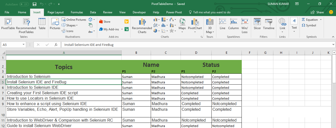
Step1: We will pick a excel file with some sample data, click here to download
Step2: Select any active cell from data set and go to insert tab :
Step3: Click on Pivot table option as shown below 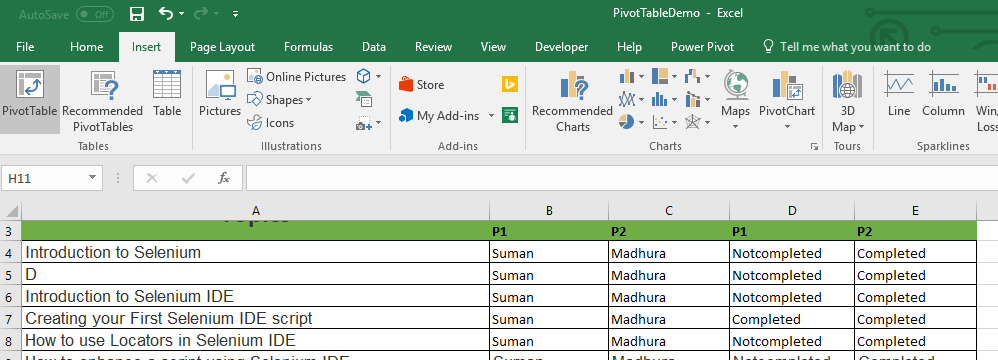
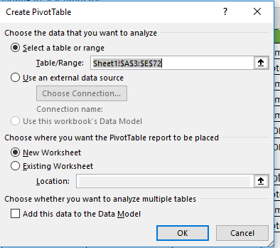
Step4: Select range for pivot table as shown below-
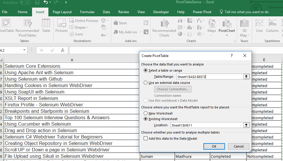
Step5 Select new worksheet for PivotTable report
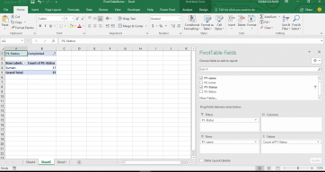
Step6: Now select he field as per requirement, for example here I want to see the number of topics completed by Suman.
P1- Name I have added in in Rows section and P1- status into summation section.

Basic summary table is ready now, we will cover more in next article about Pivot table.
I conceive this web site has got some real good information for everyone
With thanks! Valuable information!
With thanks! Valuable information!
With thanks! Valuable information!
With thanks! Valuable information!
With thanks! Valuable information!
With thanks! Valuable information!
What’s up, after reading this awesome piece http://bnuphoto.com
I got what you mean,saved to fav, very decent site. https://bzp65.com/
good stuff. I will make sure to bookmark your blog. https://miso7700.com/
It?s hard to come by knowledgeable people on this subject, however, you http://casinossir.com
good stuff. I will make sure to bookmark your blog. https://bzp65.com/
Thank you so much, will come up with more stuff like this.
I conceive this web site has got some real good information for everyone https://bzp65.com/
I have been checking out many of your stories and i can state pretty https://bzp65.com/
It?s hard to come by knowledgeable people on this subject, however, you
I got what you mean,saved to fav, very decent site. https://php665.com/
sound like you know what you?re talking about! Thanks
of writing i am as well delighted to share my know-how here with colleagues. https://newone2017.com/
With thanks! Valuable information!
thank you
good stuff. I will make sure to bookmark your blog.
thanks
I have been checking out many of your stories and i can state pretty
thanks
What’s up, after reading this awesome piece
With thanks! Valuable information!
With thanks! Valuable information!
You make more sense than the usual…
Appreciate this post. Let me try it out.